Select Processor
Select Application
Quantitative Finance
Deep Learning
(All deep learning applications have been implemented using Nvidia’s TensorFlow NGC Docker container.)
Benchmark Description
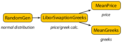
This application prices a portfolio of LIBOR swaptions on a LIBOR Market Model using a Monte-Carlo simulation. It also computes Greeks.
In each Monte-Carlo path, the LIBOR forward rates are generated randomly at all required maturities following the LIBOR Market Model, starting from the initial LIBOR rates. The swaption portfolio payoff is then computed and discounted to the pricing date. Averaging the per-path prices gives the final net present value of the portfolio.
The full algorithm is illustrated in the processing graph below:

More details can be found in Prof. Mike Giles’ notes [1].
This benchmark uses a portfolio of 15 swaptions with maturities between 4 and 40 years and 80 forward rates (and hence 80 delta Greeks). To study the performance, the number of Monte-Carlo paths is varied between 128K-2,048K.
[1] M. Giles, “Monte Carlo evaluation of sensitivities in computational finance,” HERCMA Conference, Athens, Sep. 2007.
- Application Class: Pricer
- Model: Libor Market Model
- Instrument Type: Swaption Portfolio
- Numerical Method: Monte-Carlo
- Portfolio Size: 15 swaptions
- Maturities: 4 to 40 years
- Number of Forward Rates: 80
- Number of Sensitivities: 80
- Monte-Carlo Paths:128K–1,024K
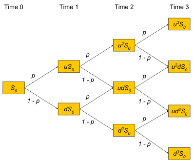
This benchmark application prices a portfolio of American call options using a Binomial lattice (Cox, Ross and Rubenstein method).
For a given size N of the binomial tree, the option payoff at the N leaf nodes is computed first (the value at maturity for different stock prices, using the Black-Scholes model). Then, the pricer works towards the root node backwards in time, multiplying the 2 child nodes by the pre-computed pseudo-probabilities that the price goes up or down, including discounting at the risk-free rate, and adding the results. After repeating this process for all time steps, the root node holds the present value.
The algorithm is illustrated in the graph below:

This binomial pricing method is applied for every option in the portfolio.
For this benchmark, we use 1,024 steps (the depth of the tree). We vary the number of options in the portfolio to study the performance.
- Application Class: Batch Pricer
- Model: Black-Scholes
- Instrument Type: American Option
- Numerical Method: Binomial Lattice
- Portfolio Size: 128K–2,048K
- Maturities: 1–5 years
- Depth of Lattice: 1,024
This benchmark application prices a portfolio of European options using the Black-Scholes-Merton formula.
The pricer calculates both the call and put price for a batch of options, defined by their current stock price, strike price, and maturities. It applies the Black-Scholes-Merton forumla for each option in the portfolio.
For this benchmark, we repeat the application of the formula 100 times to increase the overall runtime for the performance measurements. The number of options in the portfolio is varied to study the performance.
- Application Class: Batch Pricer
- Model: Black-Scholes
- Instrument Type: European Option
- Numerical Method: Closed-form Formula
- Portfolio Size: 32M-256M
- Maturities: 1–5 years
This application benchmarks the training of a deep Recurrent Neural Network (RNN), as illustrated below.
RNNs are at the core of many deep learning applications in finance, as they show excellent predition performance for time-series data.
For benchmark purposes, we focus on a single layer of such network, as this is the fundamental building block of more complex deep RNN models. We use Tensorflow, optimised by Nvidia in their NGC Docker container.
- Application Class: Deep Learning
- Model: Recurrent Neural Network (RNN)
- Mode: Training
- Hidden Layers: 1
- Hidden Units: 1,024
- Sequence Length: 32
- Batch Size: 128
- Optimizer: Stochastic gradient descent
- Training Data: Random
This application benchmarks the inference performance of a deep Recurrent Neural Network (RNN), as illustrated below.
RNNs are at the core of many deep learning applications in finance, as they show excellent predition performance for time-series data.
For benchmark purposes, we focus on a single layer of such network, as this is the fundamental building block of more complex deep RNN models. We use Tensorflow, optimised by Nvidia in their NGC Docker container.
- Application Class: Deep Learning
- Model: Recurrent Neural Network (RNN)
- Mode: Inference
- Hidden Layers: 1
- Hidden Units: 1,024
- Sequence Length: 32
This application benchmarks the training of a deep Long-Short Term Memory Model Network (LSTM). This is a modified version of the vanialla RNN, to overcome problems with vanishing or exploding gradients during back-propagation. This allows LSTMs to learn complex long-term dependencies better than RNNs.
RNNs are at the core of many deep learning applications in finance, as they show excellent predition performance for time-series data. In fact, LSTMs are often the perferred form of RNN networks in practial applications.
For benchmark purposes, we focus on a single layer of such network, as this is the fundamental building block of more complex deep LSTM models. We use Tensorflow, optimised by Nvidia in their NGC Docker container.
- Application Class: Deep Learning
- Model: Long Short Term Memory (LSTM)
- Mode: Training
- Hidden Layers: 1
- Hidden Units: 1,024
- Sequence Length: 32
- Batch Size: 128
- Optimizer: Stochastic gradient descent
- Training Data: Random
This application benchmarks the inference performance of a deep Long-Short Term Memory Model Network (LSTM). This is a modified version of the vanialla RNN, to overcome problems with vanishing or exploding gradients during back-propagation. This allows LSTMs to learn complex long-term dependencies better than RNNs.
RNNs are at the core of many deep learning applications in finance, as they show
excellent predition performance for time-series data. In fact, LSTMs are often the
perferred form of RNN networks in practial applications.
For benchmark purposes, we focus on a single layer of such network,
as this is the fundamental building block of more complex deep LSTM models.
We use Tensorflow, optimised by Nvidia in their NGC Docker container.
- Application Class: Deep Learning
- Model: Long Short Term Memory (LSTM)
- Mode: Inference
- Hidden Layers: 1
- Hidden Units: 1,024
- Sequence Length: 32
- Precision: FP16
| System | Operating System | Memory (RAM) | Compiler | ECC | Precision Mode | Other |
|---|---|---|---|---|---|---|
| Nvidia Pascal | RedHat EL 7.2 (64bit) | 256GB (host) | GCC 4.8 | on | double | max. clock boost, CUDA 8.0 |
| Intel Xeon Phi | RedHat EL 7.1 (64bit) | 64GB (host) | Intel Compiler 15.0 | on | double | MPSS 3.4.5, 4x Hyperthreading |
| System | Operating System | Memory (RAM) | Compiler | ECC | Precision Mode | Other |
|---|---|---|---|---|---|---|
| Nvidia Pascal | RedHat EL 7.4 (64bit) | 64GB (host) | GCC 4.8 | on | FP16 | max. clock boost, NGC TensorFlow 17.11 |
| System | Operating System | Memory (RAM) | Compiler | ECC | Precision Mode | Other |
|---|---|---|---|---|---|---|
| Nvidia Pascal | RedHat EL 7.4 (64bit) | 64GB (host) | GCC 4.8 | on | FP16 | max. clock boost, NGC TensorFlow 17.11 |
| System | Operating System | Memory (RAM) | Compiler | ECC | Precision Mode | Other |
|---|---|---|---|---|---|---|
| Nvidia Pascal | RedHat EL 7.4 (64bit) | 64GB (host) | GCC 4.8 | on | FP16 | max. clock boost, NGC TensorFlow 17.11 |
| System | Operating System | Memory (RAM) | Compiler | ECC | Precision Mode | Other |
|---|---|---|---|---|---|---|
| Nvidia Pascal | RedHat EL 7.4 (64bit) | 64GB (host) | GCC 4.8 | on | FP16 | max. clock boost, NGC TensorFlow 17.11 |
Hardware Specification
| Processor | Cores | Logical Cores | Frequency | GFLOPs (double) | Max. Memory | Max. Memory B/W |
|---|---|---|---|---|---|---|
| NVIDIA Tesla P100 GPU (Pascal) | 56 (SM) | 3,584 (CUDA cores) | 1,126 MHz | 4,670 | 16 GB | 720 GB/s |
| Intel Xeon Phi 7120P (Knight's Corner) | 61 | 244 | 1.238 GHz | 1,208 | 16 GB | 352 GB/s |
| Processor | Cores | Logical Cores | Frequency | GFLOPs (FP64) | GFLOPs (FP32) | GFLOPs (FP16/Tensor) | Max. Memory | Max. Memory B/W |
|---|---|---|---|---|---|---|---|---|
| NVIDIA Tesla P100 PCIe (Pascal) | 56 (SM) | 3,584 (CUDA cores) | 1,126 MHz | 4,670 | 9,340 | 18,680 | 16 GB | 720 GB/s |
| Processor | Cores | Logical Cores | Frequency | GFLOPs (FP64) | GFLOPs (FP32) | GFLOPs (FP16/Tensor) | Max. Memory | Max. Memory B/W |
|---|---|---|---|---|---|---|---|---|
| NVIDIA Tesla P100 PCIe (Pascal) | 56 (SM) | 3,584 (CUDA cores) | 1,126 MHz | 4,670 | 9,340 | 18,680 | 16 GB | 720 GB/s |
| Processor | Cores | Logical Cores | Frequency | GFLOPs (FP64) | GFLOPs (FP32) | GFLOPs (FP16/Tensor) | Max. Memory | Max. Memory B/W |
|---|---|---|---|---|---|---|---|---|
| NVIDIA Tesla P100 PCIe (Pascal) | 56 (SM) | 3,584 (CUDA cores) | 1,126 MHz | 4,670 | 9,340 | 18,680 | 16 GB | 720 GB/s |
| Processor | Cores | Logical Cores | Frequency | GFLOPs (FP64) | GFLOPs (FP32) | GFLOPs (FP16/Tensor) | Max. Memory | Max. Memory B/W |
|---|---|---|---|---|---|---|---|---|
| NVIDIA Tesla P100 PCIe (Pascal) | 56 (SM) | 3,584 (CUDA cores) | 1,126 MHz | 4,670 | 9,340 | 18,680 | 16 GB | 720 GB/s |
Speedup vs. Sequential*
(higher is better)
*the sequential version runs on a single core of an Intel Xeon E5-2698 v3 CPU
Speedup vs. Sequential*
(higher is better)
*the sequential version runs on a single core of an Intel Xeon E5-2698 v3 CPU
Speedup vs. Sequential*
(higher is better)
*the sequential version runs on a single core of an Intel Xeon E5-2698 v3 CPU
Speedup vs. P100*
(higher is better)
*the results are normalised to the P100 GPU performance
Speedup vs. P100*
(higher is better)
*the results are normalised to the P100 GPU performance
Speedup vs. P100*
(higher is better)
*the results are normalised to the P100 GPU performance
Speedup vs. P100*
(higher is better)
*the results are normalised to the P100 GPU performance
Request the Source Code

